Five key points
- R is a powerful tool for data analysis, but it can be intimidating for beginners.
- How to use R to import, explore, manipulate, model, and evaluate data using various functions and packages.
- How to use functions from the tidyverse, stats, car, broom, and caret packages to perform different tasks in data analysis.
- Predicts life expectancy based on GDP per capita and continent using regression models.
- The complete code and dataset for this project are on rstudiodatalab.com.

Data Analysis in R: A Beginner's Guide + Build a Predictive Project
R is a robust data analysis tool that can be intimidating for beginners. If you want to learn how to use R to analyze data, this article is for you. In this article, you will learn:- How to import data into R
- How to explore data using descriptive statistics and visualization
- How to manipulate data using dplyr
- How to create predictive models using regression
- How to evaluate and improve your models
After this article, you will have a reasonable basis for data analysis using R. You will also have a portfolio-worthy project to offer prospective employers or clients.
Importing Data into R
Before you can analyze data in R, import it from a source. There are several ways to import data into R, depending on the type and location of the data. For example, you may use the read.csv() method to read data from a CSV file or the read_excel() function to read data from an Excel file.
For this article, we will use a dataset from the Gapminder project, which contains information about countries' life expectancy, GDP per capita, population, and other indicators over time.
To import the dataset into R, you can use the following code:
# Load the readr package
library(readr)
# Import the dataset
gapminder <- gapminder.csv="" pre="" read_csv="">
Exploring Data with Descriptive Statistics and Visualization
Once you have imported the data into R, you must explore it to understand its structure, distribution, and relationships. Exploratory data analysis (EDA) is crucial for any data analysis project.
Two main ways to explore data in R are descriptive statistics and visualization.
- Descriptive statistics are numerical data summaries, such as mean, median, standard deviation, minimum, maximum, etc. They help you understand the central tendency, variability, and range of the data.
- Visualization is a graphical representation of the data, such as histograms, boxplots, scatterplots, etc. They help you see the data's shape, outliers, patterns, and trends.
Descriptive Statistics
To perform EDA in R, you can use functions from the tidyverse packages. The tidyverse is a collection of packages that make data analysis more accessible and more consistent in R. Some of the most valuable packages for EDA are:
- dplyr: for data manipulation
- ggplot2: for data visualization
- tidyr: for data tidying
- tibble: for creating and working with tibbles (a modern version of data frames)
To load these packages into R, you can use the following code:
# Load the tidyverse packages
library(tidyverse)
To see the structure of the gapminder dataset, you can use the str() function:
# See the structure of the
dataset
str(gapminder)
It will show you the names and types of the variables in the dataset and some sample values.
To see a summary of the dataset, you can use the summary() function:
# See a summary of the dataset
summary(gapminder)
It will show you some descriptive statistics for each variable in the dataset.
To see a glimpse of the dataset, you can use the glimpse() function from tibble:
# See a glimpse of the dataset
glimpse(gapminder)
It will show you a more compact and informative view of the dataset.
To see a sample of rows from the dataset, you can use the head() function:
 # See a sample of rows from the dataset
head(gapminder)
It will show you the first six rows of the dataset by default. You can change this by specifying a different number inside the parentheses.
To see how many rows and columns are in the dataset, you can use the dim() function:
 # See how many rows and columns
are in the dataset
dim(gapminder)
It will show you a vector with two elements: the number of rows and columns.
To see how many unique values are in each variable, you can use the n_distinct() function from dplyr:
# See how many unique values are
in each variable
n_distinct(gapminder$country) # Number of unique countries
n_distinct(gapminder$continent) # Number of unique continents
n_distinct(gapminder$year) # Number of unique years
Run this code and explore the output
It will show you the number of distinct values in each variable.
Data Visualization
To see the distribution of a numeric variable, you can use the hist() function to create a histogram:
# See the distribution of life expectancy
hist(gapminder$lifeExp)

It will show you a histogram of the life expectancy variable, which shows how many observations fall into different bins.
To see the distribution of a categorical variable, you can use the barplot() function to create a bar plot:
 # See the distribution of continent
barplot(table(gapminder$continent))

It will show you a bar plot of the continent variable, which shows how many observations belong to each category.
You may use the plot() method to build a scatterplot to observe the relationship between two numerical variables:
 # See the relationship between GDP per capita and life
expectancy
plot(gapminder$gdpPercap, gapminder$lifeExp)
It will show you a scatterplot of the GDP per capita and life expectancy variables, showing how they vary.
To see the relationship between a numeric and a categorical variable, you can use the boxplot() function to create a box plot:
 # See the relationship between continent and life expectancy
boxplot(lifeExp ~ continent, data = gapminder)

It will show you a box plot of the life expectancy variable by continent, which shows how they differ across groups.
To see the relationship between two categorical variables, you can use the mosaicplot() function to create a mosaic plot:
 # See the relationship between continent and year
mosaicplot(table(gapminder$continent, gapminder$year))

It will show you a mosaic plot of the continent and year variables, which shows their association.
To produce more elaborate and customizable charts, you can utilize the ggplot2 software. The foundation of ggplot2 is the syntax of graphics, a technique for constructing charts using layers. To build a plot using ggplot2, you need to supply three things:
- The data and variables to plot
- The geometric object (geom) represents the data
- The aesthetic mapping (aes) defines how the variables are mapped to visual attributes
For example, to create a scatterplot of GDP per capita and life expectancy with ggplot2, you can use the following code:
 # Create a scatterplot with ggplot2
ggplot(data = gapminder, # Specify the data
       mapping = aes(x = gdpPercap, y = lifeExp)) + # Specify the variables and
mapping
geom_point() # Specify the geom 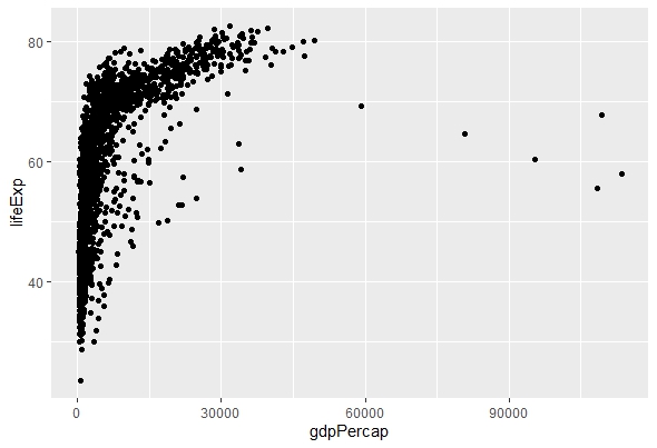
It will create a scatterplot similar to the one created with plot(), but with more options for customization. For example, you can add color, size, shape, or other attributes to your plot by adding them to the aes() function. You can add titles, labels, legends, or other elements as layers with +. You can also change the theme or scale of your plot by adding them as layers with +.
For example, to add color by continent and size by population to your scatterplot, you can use the following code:
 # Add color and size to your scatterplot
ggplot(data = gapminder,
       mapping = aes(x = gdpPercap,
                     y = lifeExp,
                     color = continent,
                     size = pop)) +
  geom_point() +
  scale_x_log10() + # Change the x-axis scale to log10
  labs(title = "GDP per capita vs Life Expectancy",
       x = "GDP per capita (log10)",
       y = "Life Expectancy",
       color = "Continent",
       size = "Population") + # Add titles and labels
theme_minimal() # Change the theme to minimal 
It will create a more informative and appealing scatterplot that shows how GDP per capita and life expectancy vary by continent and population.
There are many other geoms and options that you can use with ggplot2 to create different types of plots. You can learn more about them from here.
Manipulating Data with dplyr
After exploring your data, you can manipulate it to make it easier to analyze. For example, you may want to:
- Select or drop certain variables or observations
- Filter or subset your data based on some conditions
- Create new variables from existing ones
- Summarize or aggregate your data by groups
- Join or merge your data with other data sources
You can use functions from the dplyr package to perform these tasks in R. dplyr is a package that provides a consistent and easy-to-use set of verbs for data manipulation. Some of the most valuable functions of dplyr are:
- select(): to select or drop variables by name
- filter(): to filter or subset observations by condition
- mutate(): to create new variables from existing ones
- summarize (): to summarize or aggregate data by groups
- group_by(): to group data by one or more variables
- join(): to join or merge data with other data sources
To use these functions, you need to specify the data frame as the first argument and then the variables or conditions as the second. You can also chain multiple functions together using the pipe operator (%>%) to create a sequence of operations.
For example, to select only the country, year, and lifeExp variables from the gapminder dataset, you can use the following code:
# Select only country, year, and lifeExp
gapminder %>%
  select(country, year, lifeExp)
It will return a new data frame with only those three variables.
To filter only the observations where life expectancy is greater than 80, you can use the following code:
 # Filter only life expectancy > 80
gapminder %>%
  filter(lifeExp > 80)
It will return a new data frame with only those observations.
To create a new variable called gdp that is the product of gdpPercap and pop, you can use the following code:
# Create a new variable called gdp
gapminder %>%
  mutate(gdp = gdpPercap * pop)
It will return a new data frame with the new variable added.
To summarize the mean and standard deviation of life expectancy by continent, you can use the following code:
 # Summarize life expectancy by continent
gapminder %>%
  group_by(continent) %>% # Group by continent
  summarize(mean_lifeExp = mean(lifeExp), # Calculate mean life expectancy
            sd_lifeExp = sd(lifeExp)) # Calculate the standard deviation of life
expectancy
It will return a new data frame with the summary statistics by continent.
To join the gapminder dataset with another dataset containing information about countries' regions, you can use the following code:
Creating Predictive Models with Regression
After manipulating your data, create predictive models that can explain or forecast your outcome variable based on your predictor variables. For example, you may want to:
- Understand how GDP per capita affects life expectancy
- Predict life expectancy for a given country and year
- Compare the effects of different predictors on life expectancy
You can use functions from the stats package to perform these tasks in R. The stats package is a core package with R, providing various functions for statistical modelling and inference. Some of the most valuable functions from stats are:
- lm(): to fit linear regression models
- glm(): to fit generalized linear models
- anova(): to perform analysis of variance (ANOVA)
- summary(): to see the summary of a model fit
- predict(): to make predictions from a model fit
To use these functions, you need to specify a formula that defines the relationship between your outcome and predictor variables and then the data frame that contains those variables. You can also specify other arguments, such as weights, contrasts, or family, depending on the type of model you want to fit.
Simple Linear Regression
For example, to fit a simple linear regression model that predicts life expectancy based on GDP per capita, you can use the following code:
 # Fit a simple linear regression model
model <- a="" and="" data="" fit="" formula="" gdppercap="" lifeexp="" lm="" model="" of="" pre="" see="" specify="" summary="">
It will show you the model fit summary, including the coefficients, standard errors, p-values, R-squared, etc.
Multiple Linear Regression model
To fit a multiple linear regression model that predicts life expectancy based on GDP per capita and continent, you can use the following code:
 # Fit a multiple linear regression model
model <- a="" and="" continent="" data="" fit="" formula="" gdppercap="" lifeexp="" lm="" model="" of="" pre="" see="" specify="" summary="">
It will show you the model fit summary, including each predictor's coefficients and interactions.
Polynomial Regression Model
To fit a polynomial regression model that predicts life expectancy based on GDP per capita and its square, you can use the following code:
 # Fit a polynomial regression model
model <- and="" data="" fit="" formula="" gdppercap="" i="" lifeexp="" lm="" model="" of="" pre="" see="" specify="" summary="">
It will show you the model fit summary, including the coefficients for the linear and quadratic terms.
Logistic Regression Model
To fit a logistic regression model that predicts whether life expectancy is above or below 80 based on GDP per capita, you can use the following code:
 # Fit a logistic regression model
gapminder$lifeExp_bin <- gapminder="" ifelse="" lifeexp=""> 80, 1, 0) # Create a binary
outcome variable
model <- and="" data="" family="" fit="" formula="" gdppercap="" glm="" lifeexp_bin="" model="" of="" pre="" see="" specify="" summary="">
It will show you the model fit summary, including the coefficients, standard errors, z-values, p-values, etc.
Analysis of Variance (ANOVA)
To perform ANOVA to compare the effects of different predictors on life expectancy, you can use the following code:
 # Perform ANOVA
model1 <- a="" anova="" compare="" continent="" data="gapminder)" fit="" gdppercap="" lifeexp="" linear="" lm="" model1="" model2="" model="" models="" multiple="" pre="" regression="" simple="" the="">
It will show you the ANOVA table, including the degrees of freedom, sum of squares, mean square, F-value, and p-value for each model and their comparison.
Predictions
To make predictions from a model fit, you can use the predict() function:
 # Make predictions
newdata <- 100000="" 10000="" a="" capita="" create="" data.frame="" data="" expectancy="" fit="" frame="" from="" gdp="" gdppercap="c(1000," life="" model="" new="" newdata="" of="" per="" pre="" predict="" the="" values="" with="">
It will show you the predicted life expectancy values for the new GDP per capita. There are many other functions and options that you can use with stats to create predictive models. You can learn more about them here.
Evaluating and Improving Your Models
After creating your models, you must evaluate and improve them to ensure they are accurate and reliable. For example, you may want to:
- Check the assumptions and diagnostics of your models
- Test the significance and confidence of your models
- Compare and select the best models among different candidates
- Optimize the parameters and features of your models
To perform these tasks in R, you can use functions from various packages that provide model evaluation and improvement tools. Some of the most valuable packages are:
- car: for regression diagnostics and tests
- broom: for tidying model outputs and statistics
- caret: for classification and regression training and tuning
Required Packages
To load these packages into R, you can use the following code:
 # Load the packages for model evaluation and improvement
library(car)
library(broom)
library(caret)
Assumptions and Diagnostics of Your Models
To check the assumptions and diagnostics of your models, you can use functions from car. car provides functions for testing linearity, normality, homoscedasticity, independence, multicollinearity, outliers, leverage, influence, etc. For example,
- To test the linearity between your outcome and predictor variables, you can use the crPlots() function to create component + residual plots.
- To test the normality of your residuals (errors), you can use the qqPlot() function to create quantile-quantile plots.
- To test the homoscedasticity (equal variance) of your residuals across different values of your predictor variables, you can use the ncvTest() function to perform the Breusch-Pagan test.
- To test the independence of your residuals across different observations or groups, you can use the durbinWatsonTest() function to perform the Durbin-Watson test.
- To test multicollinearity (correlation) among your predictor variables, you can use the vif() function to calculate variance inflation factors.
- To detect outliers (extreme values) in your data or residuals, you can use the outlierTest() function to perform the Bonferroni outlier test.
- To detect leverage (influence) points in your data or residuals, you can use the hatvalues() function to calculate hat values.
- To detect influence (impact) points in your data or residuals, you can create influence plots by using the influencePlot() function.
For example,
 # Check assumptions and diagnostics of a model
model <- a="" bonferroni="" breusch-pagan="" calculate="" component="" continent="" create="" crplots="" data="gapminder)" durbin-watson="" durbinwatsontest="" factors="" fit="" gdppercap="" hat="" hatvalues="" inflation="" influence="" influenceplot="" lifeexp="" linear="" lm="" main="“Influence" model="" multiple="" ncvtest="" outlier="" outliertest="" perform="" plot="" plots="" pre="" qqplot="" quantile-quantile="" regression="" residual="" test="" values="" variance="" vif="">
It will show you the results of the tests and plots for checking the assumptions and diagnostics of the model.
Significance and Confidence of your Models
To test the significance and confidence of your models, you can use functions from stats or broom. stats provides functions for testing the overall significance of your models, such as anova() or summary(), as well as the significance of individual coefficients, such as confint() or coef(). broom provides functions for tidying the output of your models into data frames, such as tidy(), glance(), or augment(), which make it easier to work with and report your model statistics.
For example,
 # Test the significance and confidence of a model
model <- a="" and="" augment="" coefficients="" confidence="" confint="" continent="" data="" fit="" frame="" gdppercap="" glance="" intervals="" into="" lifeexp="" linear="" lm="" model="" multiple="" of="" output="" pre="" predictions="" regression="" residuals="" see="" statistics="" summary="" tidy="">
It will show you the results of the tests and data frames for testing the significance and confidence of the model.
Select the Best Models
To compare and select the best models among different candidates, you can use functions from stats or Caret. stats provides functions for comparing different models based on their statistics, such as anova() or AIC(). caret provides functions for comparing different models based on their performance metrics, such as accuracy, precision, recall, etc. For example,
 # Compare and select the best models among different
candidates
model1 <- a="" aic="" an="" and="" anova="" based="" compare="" continent="" create="" createdatapartition="" data="" fit="" for="" gapminder="" gdppercap="" i="" index="" into="" it="" lifeexp="" linear="" list="FALSE)" lm="" model1="" model2="" model3="" model="" models="" multiple="" of="" on="" p="0.8," polynomial="" pre="" regression="" reproducibility="" seed="" set.seed="" set="" sets="" simple="" split="" test="" testing="" the="" train="" train_index="" training="">
It will show you the results of the comparisons and evaluations of the different models.
To optimize the parameters and features of your models, you can use functions from Caret. Caret provides functions for tuning your models using different methods, such as grid search or random search. It also provides functions for selecting your features using different methods, such as filter methods or wrapper methods. For example,
 # Optimize parameters and features of a model
# Tune parameters of a model using grid search
model <- .="" 10-fold="" a="" and="" c="" continent="" corr="" correlated="" cross-validation="" cv="" data="train," false="" features="" filter="" for="" gdppercap="" grid="" intercept="" lifeexp="" method="lm" methods="" model.="" model="" near-zero="" number="10)," nzv="" of="" parameter="" pre="" preprocess="c(" remove="" see="" select="" selected="" the="" to="" train="" trcontrol="trainControl(method" tuned="" tunegrid="expand.grid(intercept" two="" use="" using="" values="" variance="" zero="" zv="">
It will show you the results of tuning and selecting the parameters and features of the model.
There are many other functions and options that you can use with Caret to optimize your models.
FAQs
What is R?
R is a programming language and environment for statistical computing and graphics. It is widely used by data analysts, data scientists, statisticians, and researchers.
What is the tidyverse?
The tidyverse is a collection of R packages that make data analysis easier and more consistent. It includes packages for data manipulation, visualization, tidying, modelling, and more.
What is regression?
Regression is a type of statistical modelling that aims to explain or predict an outcome variable based on one or more predictor variables. There are different regression models, such as linear regression, logistic regression, polynomial regression, etc. Read More
How do I import data into R?
There are many ways to import data into R, depending on the format and location of the data. For example, you can use the read.csv() function to read data from a CSV file or the read_excel() function to read data from an Excel file.
How do I explore data in R?
Two main ways to explore data in R are descriptive statistics and visualization. Descriptive statistics are numerical data summaries, such as mean, median, standard deviation, etc. Visualization is a graphical representation of the data, such as histograms, boxplots, scatterplots, etc.
How do I manipulate data in R?
You can use functions from the dplyr package to manipulate data in R. dplyr provides a consistent and easy-to-use set of verbs for data manipulation. Some of the most useful functions from dplyr are select(), filter(), mutate(), summarize(), group_by(), and join().
How do I create predictive models in R?
You can use functions from the stats package to create predictive models in R. The stats package provides a variety of functions for statistical modelling and inference. Some of the most valuable functions from stats are lm(), glm(), anova(), summary(), and predict().
How do I evaluate and improve my models in R?
To evaluate and improve your models in R, you can use functions from various packages that provide tools for model evaluation and improvement.
Some of the most valuable packages are car, broom, and caret. car provides functions for testing assumptions and diagnostics of your models. broom provides functions for tidying model outputs and statistics. caret provides functions for tuning and selecting your models.
Where can I find the code and dataset for this project?
You can find the complete code and dataset for this project on our website: www.rstudiodatalab.com
Where can I learn more about data analysis with R?
There are many resources to learn more about data analysis with R, such as books, courses, blogs, podcasts, etc. Some of the recommended ones are:
Conclusion
In this article, you learned how to analyze data in R using various functions and packages. You learned how to:
- Import data into R
- Explore data using descriptive statistics and visualization
- Manipulate data using dplyr
- Create predictive models using regression
- Evaluate and improve your models
You also created a portfolio-worthy project that you can showcase to potential employers or clients. You can find the complete code and dataset for this project here.
I hope you enjoyed this article and learned something new. If you have any questions or feedback, please comment below. Happy coding!
.webp)